Automating Acquisition with MATLAB® as Camera Temperature Changes

Why Change Camera Temperature During Pre-Experiment Measurements?

Before certain experiments, it is useful to take a series of measurements while key acquisition parameters change. The resultant data can then be utilized to optimize acquisition conditions. There are several situations involving temperature in which this approach may be beneficial. For example, the researcher might want to characterize the dark current of a camera so as to monitor its performance. Another situation involving temperature is when you want to ensure the best signal-to-noise ratio for an experiment whose SNR is affected by an inherent tradeoff between quantum efficiency and dark current, as is the case when working with particular wavelength ranges in the near-infrared region.

This brief document will show you how to automate data acquisition in respect to changing camera temperature using MathWorks' popular MATLAB software. In the example provided below, the dark current of a Princeton Instruments PIXIS:400BR is measured via a series of 10 sec exposures taken at discrete 5°C intervals (separated by several minutes to allow camera temperature stabilization). MATLAB is employed in conjunction with LightField, a powerful 64-bit software package that offers an intuitive interface designed specifically to control all Princeton Instruments spectrographs and cameras.

Convenient Automation Made Simple

1. Open MATLAB and initialize LightField

Each installation of LightField provides the files Setup_LightField_Environment.m" and "lfm.m".

These files can be copied into the MATLAB directory in which you are working. More details on setting up and initializing LightField from MATLAB can be found in this short video.

2. Run the following commands:

Setup_LightField_Environment
lfi = lfm(true)

Doing so will open an instance of LightField that runs in parallel to MATLAB, although you can still fully automate all functions from MATLAB while LightField runs in the background.

3. Set experiment parameters and run automated measurement.

In this step, you will be interacting with LightField to set up the experiment, set exposure times, and define a region of interest. You can also load an experiment file with default settings. Here, the following settings have been used

Exposure time: t=10s
Region of interest: Full vertical binning

4. Run the short script "temperature.m" in MATLAB. (Script can be downloaded here.)

The "temperature.m" script contains the following code:

for temp = [-70 -65 -60 -55 -50]
lfi.set(PrincetonInstruments.LightField.AddIns.CameraSettings.SensorTemperatureSetPoint,temp);
while lfi.get(PrincetonInstruments.LightField.AddIns.CameraSettings.SensorTemperatureReading)~=temp
pause(1)
end
pause(600)
data = lfi.acquire()
end

Note: All data is saved automatically via LightField's default settings. In addition, an array with spectral data is readily available in MATLAB for (automated) post-processing.

Data & Results

Figure 1 displays the dark current spectra acquired using the automation procedure detailed in the preceding section. The change in the camera's dark current performance as a function of temperature is clearly visible

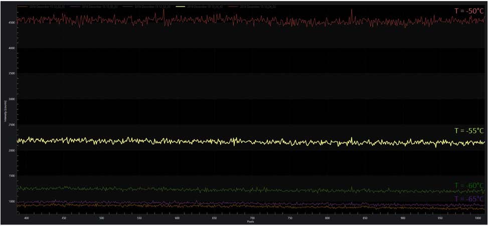
Figure 1. Dark current spectra for a backilluminated, deep-depletion CCD camera (PIXIS:400BR)

Figure 2 presents the statistical mean of measured dark current vs. temperature. The camera's dark current increases exponentially as the temperature rises.

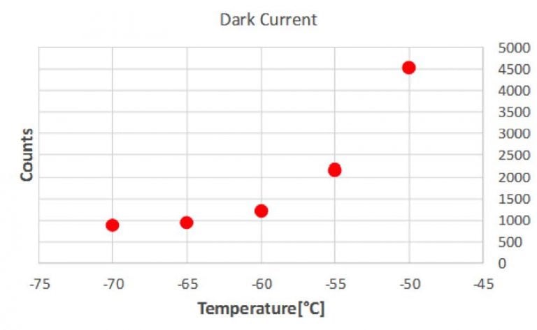
Figure 2. Spectral data from Figure 1 plotted to render
statistical meanof measured dark current vs. temperature.

For more information, please visit the LightField software page or contact us to speak to a Teledyne Princeton Instruments' representative.

Download Article as PDF

Contact An Expert